TNM112 – Teaching Session 1
Table of contents
Training Neural Network from Scratch
In this teaching session, we will build on our learning from the lab00(Introduction to Python) and create a simple neural network from scratch and see how different components of neural network training works using numpy.
Task 1: Define a Single Neuron
In this task, we’ll create a single neuron that takes 4 features [x1, x2, x3, x4] as input and produces a single output value.
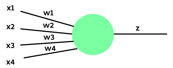
Implement the above neuron in the next cell. Follow the equations given below to compute the value of Z, followed by the output of the neuron through ReLU activation function.
\[Z = X W^\intercal + B =\begin{bmatrix} x1 & x2 & x3 & x4 \end{bmatrix} \begin{bmatrix} w1 & w2 & w3 & w4 \end{bmatrix}^\intercal + [b1],\] \[output = relu(Z)\]import numpy as np
np.random.seed(4)
# Step1: Define a function for neuron that accepts x and return z = Wxᵀ+b
def neurons(x,W,B):
# Perform the operation Wᵀx + B
return np.matmul(x,np.transpose(W)) + B
# Step2: Define a function that accepts an array and applies relu activation
def activation(x):
return np.maximum(0, x)
# Step3: Initialise Weights and biases
W = np.random.randn(1,4)
B = np.random.randn(1)
# Testing the neuron with sample input
input_vector = np.random.normal(loc=0, scale=1, size=(1,4))  # Random input vector
Z = neurons(input_vector, W, B)
output = activation(Z)

# Print the input and output
print("Input:", input_vector)
print("Weights:", W)
print("Bias Term:", B)
print("Z:", Z)
print("Output:", output)
Task 2: Add another Neuron
Now, let’s add one more neuron to this layer.
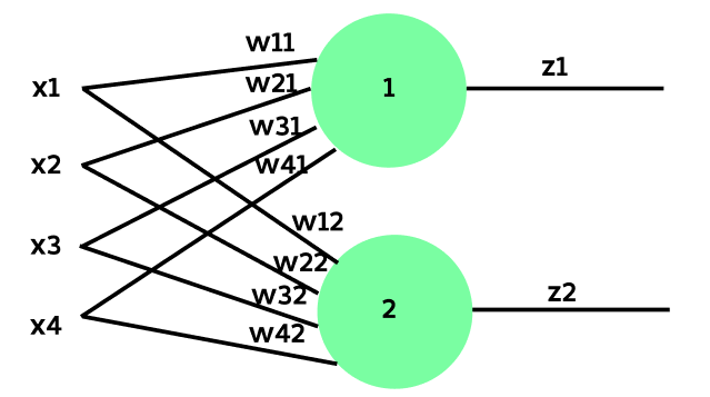
Implement the above layer of neuron in the next cell by following the equations given below. Rather than performing the calculations separately, we’ll concatenate the weights of the second neuron into the same weight matrix W as shown below:
\[Z = X W^\intercal + B = \begin{bmatrix} x1 & x2 & x3 & x4 \end{bmatrix} \begin{bmatrix} w11 & w21 & w31 & w41 \\ w12 & w22 & w32 & w42\end{bmatrix}^\intercal + \begin{bmatrix}b1 & b2\end{bmatrix},\] \[output = relu(Z)\]Note: In my setup, W has dimensions [N x M] and X has dimensions [L x M], where:
- N is the number of neurons,
- M is the number of input features for the layer,
- L is the dataset length or number of inputs.
Given these shapes, the calculation of \(Z\) will be \(X W^\intercal + B\). Some textbooks, however, may represent this calculation as \(W X + B\). Ultimately, it’s still a matrix multiplication, so just ensure the matrix dimensions are aligned accordingly.
# Step1: Initialise Weights W = [[w11, w21, w31, w41],[w12, w22, w32, w42]] and bias B = [b1, b2]
np.random.seed(4)
W = np.random.randn(2,4)
B = np.random.randn(1,2)
# Testing the neurons with sample input
input_vector = np.random.normal(loc=0, scale=1, size=(1,4))
Z = neurons(input_vector, W, B)
output = activation(Z)

# Print the input and output
print("Input:", input_vector)
print("Weights:", W)
print("Bias Term:", B)
print("Z:", Z)
print("Output:", output)
Task 3: Build a Neural Network
Previously, we explored how to create a layer with multiple neurons. Now, let’s build a simple neural network as illustrated in the figure below:
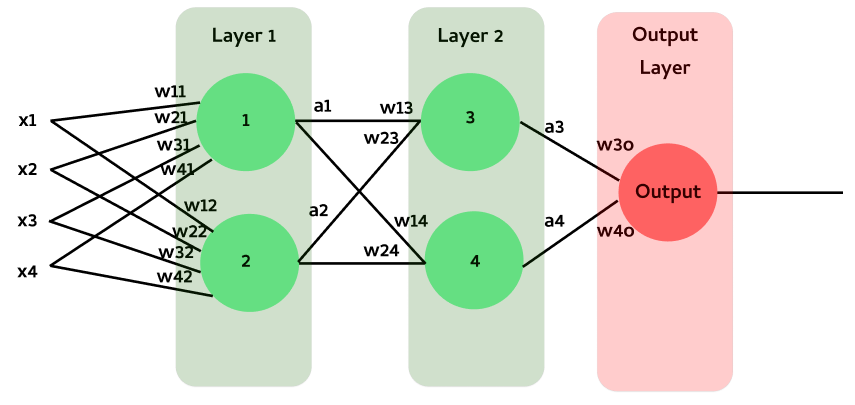
Write your implementation on the computations performed at each layer, as defined by the equations below. Step-by-step instructions are included in the comments to give you a clearer understanding.
Layer 1:
\(Z₁ = X W₁^\intercal + B₁ = \begin{bmatrix} x1 & x2 & x3 & x4 \end{bmatrix} \begin{bmatrix} w11 & w21 & w31 & w41 \\ w12 & w22 & w32 & w42\end{bmatrix}^\intercal + \begin{bmatrix}b1 & b2\end{bmatrix},\)
\[A₁ = \begin{bmatrix}a1 & a2\end{bmatrix} = relu(Z₁)\]Layer 2:
\(Z₂ = A₁ W₂^\intercal + B₂ = \begin{bmatrix} a1 & a2 \end{bmatrix} \begin{bmatrix} w13 & w23 \\ w14 & w24\end{bmatrix}^\intercal + \begin{bmatrix}b3 & b4\end{bmatrix},\)
\[A₂ = \begin{bmatrix}a3 & a4\end{bmatrix} = relu(Z₂)\]Output Layer:
\(Z₃ = A₂ W₃^\intercal + B₃ = \begin{bmatrix} a3 & a4 \end{bmatrix} \begin{bmatrix} w3o & w4o \end{bmatrix}^\intercal + \begin{bmatrix}bo\end{bmatrix},\)
\[Output = sigmoid(Z₃)\]np.random.seed(4)
class SimpleNeuralNetwork:
def __init__(self,):
# Initialize weights and biases for Layer 1 (input to first hidden layer)
self.W1 = np.random.randn(2,4)
self.B1 = np.random.randn(1,2)
# Initialize weights and biases for Layer 2 (first hidden to second hidden layer)
self.W2 = np.random.randn(2, 2)
self.B2 = np.random.randn(1,2)
# Initialize weights and biases for Output Layer (second hidden to output layer)
self.W3 = np.random.randn(1, 2)
self.B3 = np.random.randn(1,)
def relu(self, z):
return np.maximum(0, z)
def sigmoid(self, z):
return 1 / (1 + np.exp(-z))
def forward(self, X):
# Layer 1 forward pass
Z1 = np.matmul(X,np.transpose(self.W1)) + self.B1
A1 = self.relu(Z1)
# Layer 2 forward pass
Z2 = np.matmul(A1,np.transpose(self.W2)) + self.B2
A2 = self.relu(Z2)
# Output layer forward pass
Z3 = np.matmul(A2,np.transpose(self.W3)) + self.B3
Z3 = Z3.flatten()
output = self.sigmoid(Z3)
return output
# Instantiate the neural network
network = SimpleNeuralNetwork()
# Testing the neural network with sample input
X = np.random.normal(loc=0, scale=1, size=(1,4))

# Perform a forward pass
output = network.forward(X)
print("Output:", output)
Task 4 Dataset Creation
Let us create a dataset suitable for training the neural network described above. We will generate the dataset similarly to what was done in lab00. Follow the steps outlined below:
x1 = [128 x 4]input arrays sampled from normal distribution with mean=1 and std=0.1. These input values belong toClass 0i.e. y1 is a zero array of length = 128.x2 = [128 x 4]input arrays sampled from normal distribution with mean=0.5 and std=0.1. These input values belong toClass 1i.e. y2 is an array of 1s with length = 128.Concatenate x1 and x2 into X (which is the input data) and y1 and y2 into Y (which is the output data). Perform a data shuffle through indices
Follow the instructions in the comments to create the dataset.
class MyDataset:
    def __init__(self):
        # Generate data samples
        self.data, self.labels = self._generate_data()

    def _generate_data(self):
        # Generate samples for Class 0
        x1 = np.random.normal(loc=1.0, scale=0.1, size=(128, 4))
        y1 = np.zeros((128, 1), dtype=int)

        # Generate samples for Class 1
        x2 = np.random.normal(loc=0.5, scale=0.1, size=(128, 4))
        y2 = np.ones((128, 1), dtype=int)

        # Concatenate data and labels
        data = np.vstack((x1, x2))
        labels = np.vstack((y1, y2)).flatten()

        return data, labels

    def __getitem__(self, idx):
        return self.data[idx], self.labels[idx]

    def __len__(self):
        return len(self.labels)


class DataLoader:
    def __init__(self, dataset, batch_size=32, shuffle=True):
        self.dataset = dataset
        self.batch_size = batch_size
        self.shuffle = shuffle
        self.indices = np.arange(len(self.dataset))
        if self.shuffle:
            np.random.shuffle(self.indices)

    def __iter__(self):
        for start_idx in range(0, len(self.dataset), self.batch_size):
            batch_indices = self.indices[start_idx:start_idx + self.batch_size]
            batch_data = [self.dataset[i] for i in batch_indices]
            data, labels = zip(*batch_data)
            yield np.array(data), np.array(labels)

    def __len__(self):
        return int(np.ceil(len(self.dataset) / self.batch_size))

dataset = MyDataset()
dataloader = DataLoader(dataset, batch_size=32, shuffle=True)

print(f'Number of Input Data: {len(dataset)}\nNumber of Batches: {len(dataloader)}')
Task 5: Batch Computation
From task 1 to task 3, we have worked with the neural network using a single input [1 x 4] vector. Now, let’s see if it can handle a batch of input vectors [b.s x 4], where b.s is batch size (32 in this instance).
# Initialize the Dataset and use the first batch
dataset = MyDataset()
dataloader = DataLoader(dataset, batch_size=32, shuffle=True)
first_batch_data, first_batch_labels = next(iter(dataloader))

print("Shape of first batch data:\n", first_batch_data.shape)
print("Shape of first batch labels:\n", first_batch_labels.shape)

# Instantiate the neural network
network = SimpleNeuralNetwork()
output = network.forward(first_batch_data)
print("Output:", output.shape)
Task 6: Backpropagation
The backward() calculates the gradients of the loss function with respect to the weights and biases using backpropagation.
Output Layer:
The first step is to compute the error at the output layer:
\[dZ_3 = (\text{output} - y_{\text{true}}) \cdot \sigma'(Z_3)\]where \(y_{\text{true}}\) is the true label and \(\sigma'(z)\) is the derivative of the sigmoid function:
\[\sigma'(z) = \sigma(z) \cdot (1 - \sigma(z))\]The gradients for the weights and biases of the output layer are calculated as:
\[dW_3 = dZ_3^T A_2\] \[dB_3 = \sum dZ_3\]Layer 2:
To calculate the error propagated back to the second hidden layer:
\[dA_2 = dZ_3 W_3^T\] \[dZ_2 = dA_2 \cdot \text{ReLU}'(Z_2)\]where \(\text{ReLU}'(z)\) is defined as:
\[\text{ReLU}'(z) = \begin{cases} 1 & \text{if } z > 0 \\ 0 & \text{if } z \leq 0 \end{cases}\]The gradients for the weights and biases of the second hidden layer are:
\[dW_2 = dZ_2^T A_1\] \[dB_2 = \sum dZ_2\]Layer 1:
To calculate the error propagated back to the first hidden layer:
\[dA_1 = dZ_2 W_2^T\] \[dZ_1 = dA_1 \cdot \text{ReLU}'(Z_1)\]The gradients for the weights and biases of the first hidden layer are:
\[dW_1 = dZ_1^T X\] \[dB_1 = \sum dZ_1\]Updating Weights and Biases:
Finally, the weights and biases are updated using gradient descent:
\(W_3 \leftarrow W_3 - \eta dW_3\) \(B_3 \leftarrow B_3 - \eta dB_3\)
\(W_2 \leftarrow W_2 - \eta dW_2\) \(B_2 \leftarrow B_2 - \eta dB_2\)
\(W_1 \leftarrow W_1 - \eta dW_1\) \(B_1 \leftarrow B_1 - \eta dB_1\)
where \(\eta\) is the learning rate.
import numpy as np

class SimpleNeuralNetwork:
    def __init__(self):
        # Initialize weights and biases for Layer 1 (input to first hidden layer)
        self.W1 = np.random.randn(2, 4)  # (2 neurons, 4 features)
        self.B1 = np.random.randn(1, 2)   # (1, 2 neurons)

        # Initialize weights and biases for Layer 2 (first hidden to second hidden layer)
        self.W2 = np.random.randn(2, 2)   # (2 neurons, 2 neurons)
        self.B2 = np.random.randn(1, 2)   # (1, 2 neurons)

        # Initialize weights and biases for Output Layer (second hidden to output layer)
        self.W3 = np.random.randn(1, 2)   # (1 output, 2 neurons)
        self.B3 = np.random.randn(1,)      # (1 output)

    def relu(self, z):
        return np.maximum(0, z)

    def sigmoid(self, z):
        return 1 / (1 + np.exp(-z))

    def relu_derivative(self, z):
        return (z > 0).astype(float)

    def sigmoid_derivative(self, z):
        s = self.sigmoid(z)
        return s * (1 - s)

    def forward(self, X):
        # Store intermediate values for use in backpropagation
        self.X = X

        # Layer 1 forward pass
        self.Z1 = np.matmul(X, np.transpose(self.W1)) + self.B1
        self.A1 = self.relu(self.Z1)

        # Layer 2 forward pass
        self.Z2 = np.matmul(self.A1, np.transpose(self.W2)) + self.B2
        self.A2 = self.relu(self.Z2)

        # Output layer forward pass
        self.Z3 = np.matmul(self.A2, np.transpose(self.W3)) + self.B3
        self.output = self.sigmoid(self.Z3)

        return self.output

    def backward(self, y_true, learning_rate=0.01):

        # Calculate output layer error
        dZ3 = (self.output - y_true) * self.sigmoid_derivative(self.Z3)  # Output error
        dW3 = np.matmul(dZ3.T, self.A2)  # Weight gradients for W3
        dB3 = np.sum(dZ3, axis=0, keepdims=True)  # Bias gradients for B3

        # Calculate the error for Layer 2
        dA2 = np.matmul(dZ3, self.W3)  # Propagate the error backward
        dZ2 = dA2 * self.relu_derivative(self.Z2)  # Apply ReLU derivative
        dW2 = np.matmul(dZ2.T, self.A1)  # Weight gradients for W2
        dB2 = np.sum(dZ2, axis=0, keepdims=True)  # Bias gradients for B2

        # Calculate the error for Layer 1
        dA1 = np.matmul(dZ2, self.W2)  # Propagate the error backward
        dZ1 = dA1 * self.relu_derivative(self.Z1)  # Apply ReLU derivative
        dW1 = np.matmul(dZ1.T, self.X)  # Weight gradients for W1
        dB1 = np.sum(dZ1, axis=0, keepdims=True)  # Bias gradients for B1

        # Update weights and biases
        self.W3 -= learning_rate * dW3
        self.B3 -= learning_rate * dB3.flatten()
        self.W2 -= learning_rate * dW2
        self.B2 -= learning_rate * dB2.flatten()
        self.W1 -= learning_rate * dW1
        self.B1 -= learning_rate * dB1.flatten()
np.random.seed(4)

# Initialize the Dataset
dataset = MyDataset()
dataloader = DataLoader(dataset, batch_size=32, shuffle=True)
model = SimpleNeuralNetwork()

# Do batch computation over the dataset
print(f"Epoch 1:")
print("===============================================")
for batch_idx, (data, labels) in enumerate(dataloader):
    # Forward pass
        outputs = model.forward(data)
        labels = labels[:, np.newaxis]

        # Compute the loss (Mean Squared Error for simplicity here)
        loss = np.mean((outputs - labels) ** 2)

        # Print the loss for every batch
        print(f"Batch {batch_idx + 1} - Loss: {loss}\n")

        # Backward pass and update weights
        model.backward(labels)
Task 7: Training (Optional)
Increase the number of data in the dataset (from 256x4 to 1024x4, where each class labels has 512x4) and train the above network for more number of epochs and check whether the loss is decreasing.
#Implement your code here